Tidyverse

https://www.tidyverse.org/

Tidyverse

The tidyverse is a collection of packages based on 4 principles for handling data:

1. Reuse existing data structures
2. Compose simple functions with the pipe
3. Embrace functional programming
4. Design for humans

The R project for Statistical Computing was built for a different age; the tidyverse is a collection of tools for our age

The tidy tools manifesto

Base R functions for read-write the data

• scan() - Read data into a vector or list from the console or file

• read.table(), read.csv(), read.delim() - Reads a file in table format and creates a data frame from it, with cases corresponding to lines and variables to fields in the file

• write.table(), write.csv() - Saves the object (data.frame) to a file

• ?data.table::fread for very fast data read into R

• "File -> Import Dataset" in RStudio

readr

• There are some built-in functions for reading in data in text files. These functions are read-dot-something, for example, read.csv() reads in comma-delimited text data; read.delim() reads in tab-delimited text, etc.

• readr package provides fast and intelligent data reading capabilities. Very similar looking functions, named read-underscore-something -- e.g., read_csv()

• They're good at guessing the types of data in the columns, they don't do some of the other silly things that the base functions do

• Play nicely with dplyr - data manipulation package

http://readr.tidyverse.org/

tibbles

Data frames are great! Except for

• printing them
• working with both characters and factors
• manipulating multiple columns
• You need to remember to set options(stringsAsFactors = FALSE)
• If you want a one-collumn data frame, you need to use dat[, "column1", drop = FALSE]

tibbles are the data frame alternative simplifying work with data frame-like objects

https://tibble.tidyverse.org/

tibbles

• A tibble, or tbl_df, is a modern reimagining of the data.frame, keeping what time has proven to be effective, and throwing out what is not

• Tibbles are data.frames that are lazy and surly: they do less (i.e., they don't change variable names or types, and don't do partial matching) and complain more (e.g., when a variable does not exist)

• This forces you to confront problems earlier, typically leading to cleaner, more expressive code. Tibbles also have an enhanced print method which makes them easier to use with large datasets containing complex objects

  • Hadley Wickham, Chief Scientist at RStudio

• glimpse() into tibble, analog of str()

Making the data tidy with tidyr

• Principles of tidy data
  • Each column is a variable
  • Each row is an observation

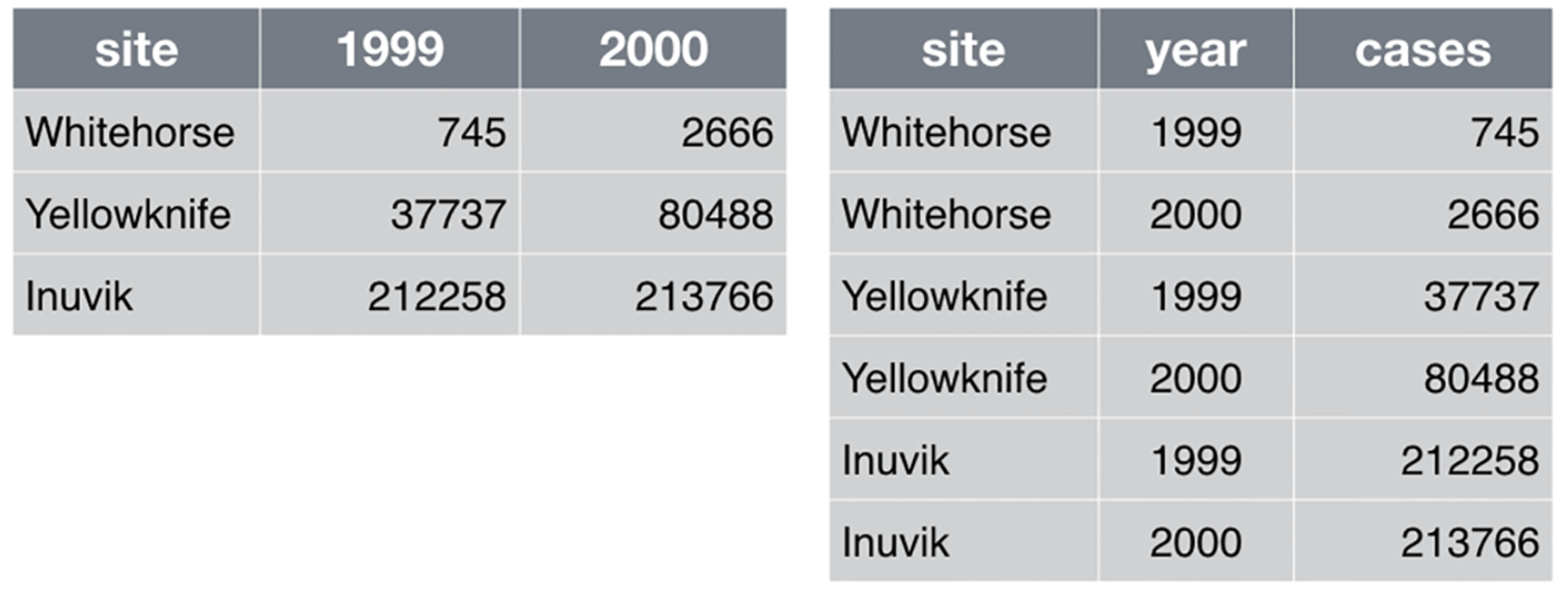
Tidy data paper, http://www.jstatsoft.org/v59/i10/paper

Making the data tidy with tidyr

• tidyr - flexible data reshaping
  • pivot_longer() - "lengthens" data, increasing the number of rows and decreasing the number of columns
  • pivot_wider() - "widens" data, increasing the number of columns and decreasing the number of rows

Example of converting the wide data into tidy data

https://tidyr.tidyverse.org/index.html, vignette("tidy-data"), vignette("pivot")

dplyr: data manipulation with R

80% of your work will be data preparation

• getting data (from databases, spreadsheets, flat-files)

• performing exploratory/diagnostic data analysis

• reshaping data

• visualizing data

dplyr: data manipulation with R

80% of your work will be data preparation

• Filtering rows (to create a subset)

• Selecting columns of data (i.e., selecting variables)

• Adding new variables

• Sorting

• Aggregating

• Joining

dplyr: A grammar of data manipulation

• The dplyr package gives you a handful of useful verbs for managing data. On their own they don't do anything that base R can't do

• Basic dplyr verbs

  • filter()
  • select()
  • mutate()
  • arrange()
  • summarize()
  • group_by()

• They all take a data frame or tibble as their input for the first argument, and they all return a data frame or tibble as output

https://dplyr.tidyverse.org/

The pipe %>% operator

• Pipe %>% output of one command into an input of another command - chain commands together. (Think about the "|" operator in Linux)
• Imported from magrittr package
• Read as "then". Take the dataset (or object), then do ...

library(dplyr)
round( sqrt(1000), 3)

## [1] 31.623

1000 %>% sqrt %>% round(., 3)

## [1] 31.623

The pipe %>% operator

• For example, we can view the head of the diamonds data.frame using either of the last two lines of code here:

library(dplyr)
library(ggplot2)
data(diamonds)
head(diamonds)
diamonds %>% head

## # A tibble: 6 x 10
##   carat cut       color clarity depth table price     x     y     z
##   <dbl> <ord>     <ord> <ord>   <dbl> <dbl> <int> <dbl> <dbl> <dbl>
## 1 0.23  Ideal     E     SI2      61.5    55   326  3.95  3.98  2.43
## 2 0.21  Premium   E     SI1      59.8    61   326  3.89  3.84  2.31
## 3 0.23  Good      E     VS1      56.9    65   327  4.05  4.07  2.31
## 4 0.290 Premium   I     VS2      62.4    58   334  4.2   4.23  2.63
## 5 0.31  Good      J     SI2      63.3    58   335  4.34  4.35  2.75
## 6 0.24  Very Good J     VVS2     62.8    57   336  3.94  3.96  2.48

The pipe %>% operator

For example, read the last line of code as: "Take the price column of the diamonds data.frame and then summarize it"

library(dplyr)
data(diamonds)
head(diamonds)
diamonds %>% head
summary(diamonds$price)
diamonds$price %>% summary(object = .)

• There's a keyboard shortcut to insert the %>% sequence - you can see what it is by clicking the Tools menu in RStudio, then selecting Keyboard Shortcut Help
• On Mac, it's CMD-SHIFT-M

dplyr::filter()

If you want to filter rows of the data where some condition is true, use the filter() function.

1. The first argument is the data frame you want to filter, e.g. filter(mydata, ....
2. The second argument is a condition you must satisfy, e.g. filter(ydat, symbol == "LEU1"). If you want to satisfy all of multiple conditions, you can use the "and" operator, &. The "or" operator | (the pipe character, usually shift-backslash) will return a subset that meet any of the conditions.

• ==: Equal to
• !=: Not equal to
• >, >=: Greater than, greater than or equal to
• <, <=: Less than, less than or equal to

dplyr::filter()

For example, keep only the entries with Ideal cut

df.diamonds_ideal <- filter(diamonds, cut == "Ideal")
df.diamonds_ideal

## # A tibble: 21,551 x 10
##    carat cut   color clarity depth table price     x     y     z
##    <dbl> <ord> <ord> <ord>   <dbl> <dbl> <int> <dbl> <dbl> <dbl>
##  1  0.23 Ideal E     SI2      61.5    55   326  3.95  3.98  2.43
##  2  0.23 Ideal J     VS1      62.8    56   340  3.93  3.9   2.46
##  3  0.31 Ideal J     SI2      62.2    54   344  4.35  4.37  2.71
##  4  0.3  Ideal I     SI2      62      54   348  4.31  4.34  2.68
##  5  0.33 Ideal I     SI2      61.8    55   403  4.49  4.51  2.78
##  6  0.33 Ideal I     SI2      61.2    56   403  4.49  4.5   2.75
##  7  0.33 Ideal J     SI1      61.1    56   403  4.49  4.55  2.76
##  8  0.23 Ideal G     VS1      61.9    54   404  3.93  3.95  2.44
##  9  0.32 Ideal I     SI1      60.9    55   404  4.45  4.48  2.72
## 10  0.3  Ideal I     SI2      61      59   405  4.3   4.33  2.63
## # … with 21,541 more rows

dplyr::filter()

We can achieve this same result using the %>% operator

diamonds %>% head
df.diamonds_ideal <- filter(diamonds, cut == "Ideal")
df.diamonds_ideal <- diamonds %>% filter(cut == "Ideal")

dplyr::select()

• The filter() function allows you to return only certain rows matching a condition. The select() function returns only certain columns. The first argument is the data, and subsequent arguments are the columns you want.
  • Syntax: select(data, columns)

df.diamonds_ideal %>% head
select(df.diamonds_ideal, carat, cut, color, price, clarity)
df.diamonds_ideal <- df.diamonds_ideal %>% select(., carat, cut, color, price, clarity)

dplyr::mutate()

• The mutate() function adds new columns to the data that are functions of old columns

• It doesn't actually modify the data frame you're operating on, and the result is transient unless you assign it to a new object or reassign it back to itself (generally, not a good practice)

  • Syntax: mutate(data, new_column = function(old_columns))

df.diamonds_ideal %>% head
mutate(df.diamonds_ideal, price_per_carat = price/carat)
df.diamonds_ideal <- df.diamonds_ideal %>% mutate(price_per_carat = price/carat)

dplyr::arrange()

• The arrange() function does what it sounds like - sorts things

• It takes a data.frame or tbl_df and arranges (or sorts) by column(s) of interest

• The first argument is the data, and subsequent arguments are columns to sort on. Use the desc() function to arrange by descending

  • Syntax: arrange(data, column_to_sort_by)

df.diamonds_ideal %>% head
arrange(df.diamonds_ideal, price)
df.diamonds_ideal %>% arrange(price, price_per_carat)

dplyr::summarize()

• The summarize() function summarizes multiple values to a single value

• The power of summarize() comes from a few convenience functions called n() and n_distinct() that tell you the number of observations or the number of distinct values of a particular variable.

  • Syntax: summarize(function_of_variables)

summarize(df.diamonds_ideal, length = n(), avg_price = mean(price))
df.diamonds_ideal %>% summarize(length = n(), avg_price = mean(price))

dplyr::group_by()

• Summarize subsets of columns by custom summary statistics

• Syntax: group_by(data, column_to_group)

group_by(diamonds, cut) %>% summarize(mean(price))
group_by(diamonds, cut, color) %>% summarize(mean(price))

The power of pipe %>%

• Summarize subsets of columns by custom summary statistics

arrange(mutate(arrange(filter(tbl_df(diamonds), cut == "Ideal"), price),
  price_per_carat = price/carat), price_per_carat)
arrange(
  mutate(
    arrange(
      filter(tbl_df(diamonds), cut == "Ideal"), 
    price), 
  price_per_carat = price/carat), 
price_per_carat)
diamonds %>% filter(cut == "Ideal") %>% arrange(price) %>%
  mutate(price_per_carat = price/carat) %>% arrange(price_per_carat)

Joining data frames

• inner_join(x, y): Keep only rows where there are observations in both x and y
• left_join(x, y): Keep all rows from x, whether they have a match in y or not (unmatched rows are filled with NAs)
• right_join(x, y): Keep all rows from y, whether they have a match in x or not
• full_join(x, y): Keep all rows from both x and y, whether they have a match in the other dataset or not

Review https://ready4r.netlify.app/labbook/part-5-doing-useful-things-with-multiple-tables.html#joining-tables

Working with factors tidyverse way

library(forcats)

• fct_rev() - Reverse order of factor levels

• fct_reorder() - Reordering a factor by another variable

• fct_collapse() - Collapse multiple categories into one category

• fct_lump() - Collapsing the least/most frequent values of a factor into “other”

• fct_infreq() - Reordering a factor by the frequency of values

• fct_relevel() - Changing the order of a factor by hand

https://forcats.tidyverse.org/